Signaux Usuels#
Cette page donne l’expression des signaux usuels et montre comment les implémenter en Python.
import numpy as np
import matplotlib.pyplot as plt

t = np.arange(-2,2,0.001)
Impulsion de Dirac#
\[\begin{split}\delta(t)=\left\{\begin{array}{cc}\infty &\text{si }t= 0\\0 &\text{ailleurs}\end{array}\right.\end{split}\]
sous la contrainte
\[\int_{-\infty}^{\infty}\delta(t)dt = 1\]
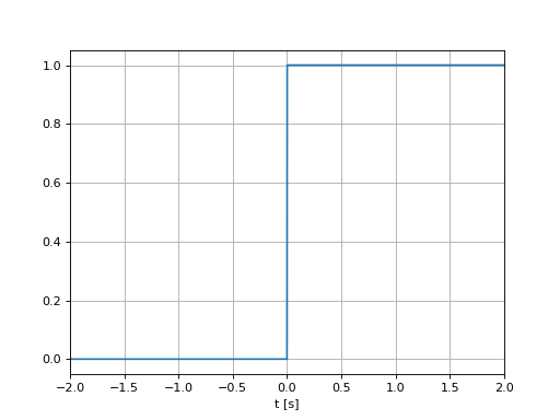
Echelon unitaire#
\[\begin{split}u(t)=\left\{\begin{array}{cc}1 &\text{si }t\ge 0\\0 &\text{ailleurs}\end{array}\right.\end{split}\]
u = (t>=0)

plt.plot(t,u)
plt.grid()
plt.xlabel("t [s]")
plt.xlim([-2,2])
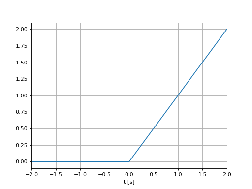
Rampe unitaire#
\[r(t)=t u(t)\]
r = t*(t>=0)

plt.plot(t,r)
plt.grid()
plt.xlabel("t [s]")
plt.xlim([-2,2])
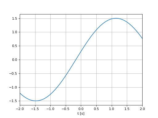
Sinsusoide#
\[x(t)=a \sin(\omega_0 t+\varphi)\]
\(\omega_0\): pulsation (rad/s),
\(a\): amplitude (crète),
\(\varphi\): déphasage.
w0, a, varphi = 1.2, 1.5, 0.2
x = a*np.sin(w0*t+varphi)

plt.plot(t,x)
plt.grid()
plt.xlabel("t [s]")
plt.xlim([-2,2])
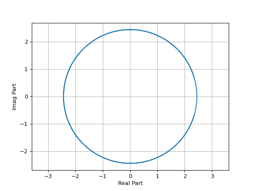
Exponentielle Complexe#
\[z(t)=a e^{j\omega t+\varphi}\]
\(\omega_0\): pulsation (rad/s),
\(a\): amplitude (crète),
\(\varphi\): déphasage.
w0, a, varphi = 3, 2, 0.2
z = a*np.exp(1j*w0*t+varphi)

plt.plot(np.real(z),np.imag(z))
plt.grid()
plt.xlabel("Real Part")
plt.ylabel("Imag Part")
plt.axis("equal")
plt.xlim([-2,2])
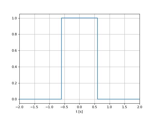
Porte rectangulaire#
\[\begin{split}\Pi_L(t)=\left\{\begin{array}{cc}1 &\text{si }|t| <\frac{L}{2}\\0 &\text{ailleurs}\end{array}\right.\end{split}\]
\(L\): largeur de la porte.
L=1.2
p = np.abs(t)< (L/2)

plt.plot(t,p)
plt.grid()
plt.xlabel("t [s]")
plt.xlim([-2,2])