Digital Oscillators#
In this tutorial, we shows how to generate a digital waveform using a lookup table. Specifically, we focus on the generation of a sine waveform, but this tutorial can be easily extended to other waveforms such as triangle or sawtooth waveforms.
Sine Wave Waveform#
A sine wave is mathematically described by :
\(f_0\) corresponds to the fundamental frequency.
In the digital domain, the sine wave can be obtained by evaluating \(x(t)\) for \(t=n/f_s\) where \(n \in \mathbb{N}\) and \(f_s\) is the sampling frequency.
When using the C language, the function \(x[n]=x(n/fs)\) can be evaluated
naively using the sin function of the library math.h. Nevertheless, it is important to note that the evaluation of trigonometric functions
has a relatively large computational cost. In this tutorial, we describe an alternative low-complexity implementation based on a wavetable oscillator.
Wavetable Oscillator#
To reduce the computational complexity, one solution is to store in memory a single full cycle of a reference waveform. For a sine wave, the reference waveform is given by :
\(N\) corresponds to the length of the wavetable.
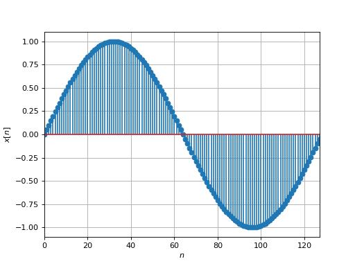
The fundamental frequency of this waveform depends on the sampling frequency f_s. By reading each sample
of the wavetable sample by sample, we can synthesize a periodic waveform with a fixed fundamental frequency :
Controlling the Fundamental Frequency#
Instead of generating a periodic signal with a fixed frequency, a synthesizer must be able to generate a periodic signal with a time varying frequencies \(f_{0}\). In this subsection, we shows how to modify the rate at which the samples are read in the wavetable to control the frequency \(f_{0}\) of the waveform.
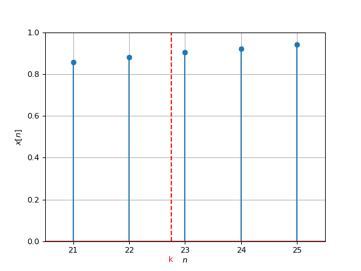
Let us denote by \(y[n]\) the \(n^{th}\) output sample and let us consider that \(y[n] = x[m]\). To synthesize a waveform with fundamental frequency \(f_{0}\), the next output sample can be expressed by :
\(\Delta=N\frac{f_0}{f_s}\) corresponds to the phase delta (increment) between two adjacent samples.
In the above expression, the next index \(k=m+\Delta\) is not always an integer as illustrated in the above figure. To obtain the value of \(x[k]\), two solutions are commonly used.
Zero order Interpolation#
When the index \(k\) is not an integer, a simple solution is to truncate the value of \(k\) to the greatest integer less than or equal to \(k\). Specifically, we can Mathematically, the next output sample is then given by :
\(\lfloor . \rfloor\) corresponds to the rounding operator. For example, \(\lfloor 3.21 \rfloor=3\) and \(\lfloor 5.98 \rfloor=5\).
Linear Interpolation#
To improve the oscillator quality, another solution is to estimate the value of \(y[n+1]\) from the two nearest samples using an interpolation algorithm. Using a linear interpolation, the next output sample can be expressed as :
\(\alpha = k-\lfloor k \rfloor\) is a weighting coefficient (\(0\le \alpha<1\)),
\(x_l=x[\lfloor k \rfloor]\) and \(x_r = x[\lfloor k \rfloor+1]\) corresponds to two adjacent samples.
C Implementation#
The following code shows a possible C implementation for the wavetable synthesizer.
void oscillator(double *buffer, double f0, int fs, double *currentIndex, int size)
{
    double coef;
    float index = *currentIndex;
    float delta = N*(f0/(1.0*fs));
    int index_l, index_r;
    int n;

    for(n=0; n<size; n++)
    {
        index_l = (int)index;
        index_r = (index_l == (N-1)) ? 0 : index_l+1;
        coef = index - index_l;
        buffer[n] = wavetable[index_l]+ coef*(wavetable[index_r]-wavetable[index_l]);
        //update increment
        index += delta;
        if (index > N)
        {
            index -= N;
        }
    }
    *currentIndex = index; //export index
}
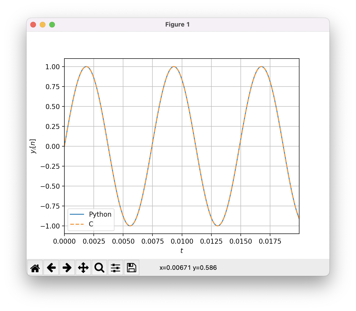
Verification#
I recommend to check the validity of the C code by comparing the output of the C and Python implementation.
First, compile the C code as a shared library
$ gcc -fPIC -shared my_lib.c -o my_lib.so
Then, run the following python code.
import ctypes
import numpy as np
from numpy.ctypeslib import ndpointer
import matplotlib.pyplot as plt
from scipy import signal

# import C function
lib = ctypes.cdll.LoadLibrary("./my_lib.so")
oscillator = lib.oscillator
oscillator.restype = None
oscillator.argtypes = [ndpointer(ctypes.c_double, flags="C_CONTIGUOUS"),
                ctypes.c_double,
                ctypes.c_size_t,
                ctypes.POINTER(ctypes.c_double),
                ctypes.c_size_t]

# parameter
fs = 44100
f0 = 134.23

# create oscillator
t = np.arange(0, 0.02, 1/fs)
x = np.sin(2*np.pi*f0*t)

# allocate arguments and call the C function
N = len(t)
y = np.zeros(N)
currentIndex = ctypes.c_double(0.0)
oscillator(y, f0, fs, ctypes.pointer(currentIndex), N)

# plot the result
plt.plot(t, x, label="Python")
plt.plot(t, y, "--", label="C")
plt.grid()
plt.xlabel("$t$")
plt.ylabel("$y_l[n]$")
plt.xlim([0,t[-1]])
plt.legend()
plt.show()
References#
JUCE C++ implementation: https://docs.juce.com/master/tutorial_wavetable_synth.html