Digital State Variable Filter#
In this tutorial, we show how to implement a parametric IIR filter. Specifically, we focus on the implementation of a digital state variable filter.
Filter Structure#
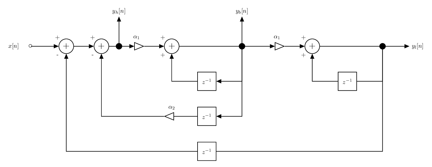
The structure of the digital state variable filter is provided below.

The state variable filter has 1 input and 3 outputs. Each output corresponds to a particular filter type:
\(y_h[n]\): high pass filter,
\(y_b[n]\): band pass filter,
\(y_l[n]\): low pass filter.
The state variable filter depends on the parameters \(\alpha_1\) and \(\alpha_2\). These two parameters are directly linked to the frequency characteristics of the filter. Specifically:
\(\alpha_1=2\sin(\pi f_c/F_s)\): where \(f_c\) is the cut-off frequency and \(F_s\) is the sampling frequency,
\(\alpha_2=1/Q\): where \(Q\) is the Q factor.
Analysis of the Low Pass Filter#
Difference equation#
The low pass filter can be described by the difference equation :
where \(a_1=\alpha_1^2+\alpha_1\alpha_2-2\) and \(a_2=1-\alpha_1\alpha_2\).
Frequency Response#
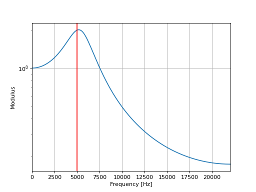
The following script plots the frequency response of the low-pass filter.
import numpy as np
import matplotlib.pyplot as plt

from scipy import signal

fc = 5000
fs = 44100
Q = 2

alpha1 = 2*np.sin(np.pi*fc/fs)
alpha2 = 1/Q

b = [alpha1**2]
a = [1, (alpha1**2+alpha1*alpha2-2), (1-alpha1*alpha2)]
f, h = signal.freqz(b, a, fs=fs)
plt.semilogy(f, abs(h))
plt.axvline(fc,c="r")
plt.grid()
plt.xlabel("Frequency [Hz]")
plt.ylabel("Modulus")
plt.xlim([0, fs/2])

C Implementation#
Block-based Implementation#
The following code shows a possible C implementation of the state variable filter. This implementation
uses a state array zi that store the previous values of \(y_b[n-1]\) and \(y_bl[n-1]\). This state
array allows to pass the filter state from block to block.
#include <math.h>

void state_variable_filter(double *buffer, double *zi, int size, double Q, double fc, int fs)
{
    // This function applies a state variable filter to the data contained in a buffer *buffer
    // zi: [y_b[n-1], y_l[n-1]]
    int i;
    double alpha1 = 2.0*sin(M_PI*fc/(1.0*fs));
    double alpha2 = 1.0/Q;
    double y_h, y_b, y_l, x;

    for(i=0; i<size; i++){
        x = buffer[i];
        y_h = x - zi[1] - alpha2*zi[0];
        y_b = alpha1*y_h + zi[0];
        y_l = alpha1*y_b + zi[1];
        buffer[i] = y_l;

        //update states
        zi[0] = y_b;
        zi[1] = y_l;
    }
}
Verification#
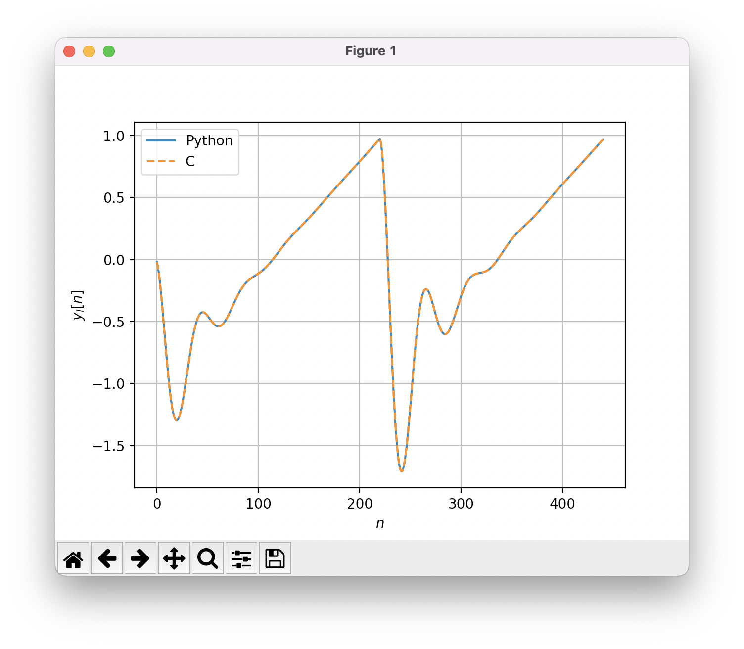
I recommend to check the validity of the C code by comparing the output of the C and Python implementation.
First, compile the C code as a shared library
$ gcc -fPIC -shared my_lib.c -o my_lib.so
Then, in the same folder, run the following python code.
import ctypes
import numpy as np
from numpy.ctypeslib import ndpointer
import matplotlib.pyplot as plt
from scipy import signal

# import C function
lib = ctypes.cdll.LoadLibrary("./my_lib.so")
state_variable_filter = lib.state_variable_filter
state_variable_filter.restype = None
state_variable_filter.argtypes = [ndpointer(ctypes.c_double, flags="C_CONTIGUOUS"),
                ndpointer(ctypes.c_double, flags="C_CONTIGUOUS"),
                ctypes.c_size_t,
                ctypes.c_double,
                ctypes.c_double,
                ctypes.c_size_t
                ]

# parameter
fs = 44100
fc = 1000
Q = 2

# create oscillator
t = np.arange(0, 0.01, 1/fs)
x = signal.sawtooth(2*np.pi*200*t)

# python code
alpha1 = 2*np.sin(np.pi*fc/fs)
alpha2 = 1/Q
b = [alpha1**2]
a = [1, alpha1**2+alpha1*alpha2-2, 1-alpha1*alpha2]
y_out = signal.lfilter(b, a, x)

# allocate arguments and call the C function
N = len(t)
zi = np.zeros(2)
buffer = x
state_variable_filter(buffer, zi, N, Q, fc, fs)

# plot the result
plt.plot(y_out, label="Python")
plt.plot(buffer, "--", label="C")
plt.grid()
plt.xlabel("$n$")
plt.ylabel("$y_l[n]$")
plt.legend()
plt.show()

References#
JUCE C++ implementation: juce-framework/JUCE
Zolzer, DAFX: Digital Audio Effects, http://www.music.mcgill.ca/~ich/classes/FiltersChap2.pdf