PAPR in OFDM Communication#
In this tutorial, we compute the Peak-to-Average Power Ratio (PAPR)
of an OFDM signal using the comnumpy library.
We reproduce the first figure from the article:
“An overview of peak-to-average power ratio reduction techniques for multicarrier transmission” by Han and Lee (2005).
You will learn how to:
Build an OFDM chain with multiple subcarriers.
Compute the PAPR of a single OFDM signal.
Evaluate the Complementary Cumulative Distribution Function (CCDF) of PAPR.
Compare simulation results with theoretical curves.
Introduction#
Import Libraries#
We start by importing the necessary libraries:
import numpy as np
import matplotlib.pyplot as plt
from tqdm import tqdm
from comnumpy.core import Sequential
from comnumpy.core.generators import SymbolGenerator
from comnumpy.core.mappers import SymbolMapper
from comnumpy.core.processors import Serial2Parallel, Parallel2Serial
from comnumpy.core.utils import get_alphabet
from comnumpy.core.metrics import compute_ccdf
from comnumpy.ofdm.processors import CarrierAllocator, IFFTProcessor
from comnumpy.ofdm.metrics import compute_PAPR

# This script reproduces the first figure of the following article :
Define Parameters#
Next, we define the simulation parameters: the number of subcarriers, modulation, oversampling factor, and thresholds for PAPR analysis.
img_dir = "../../docs/examples/img/"


# parameters
N_sc = 1024
L = 10000
type, M = "PSK", 4
alphabet = get_alphabet(type, M)
alphabet_generator = np.arange(M)
papr_dB_threshold = np.arange(4, 13, 0.1)
Here:
N_sc: number of subcarriers (1024 by default).L: number of OFDM symbols to generate.os: oversampling factor, used to better approximate the continuous-time signal.papr_dB_threshold: thresholds (in dB) for computing theoretical CCDF curves.
OFDM Communication Chain#
We now build an OFDM transmission chain using Sequential.
It includes symbol generation, mapping, serial-to-parallel conversion,
carrier allocation, and IFFT processing.
# defaut carrier type
carrier_type = np.zeros(os*N_sc)
carrier_type[:N_sc] = 1

# perform simulation
chain = Sequential([
        SymbolGenerator(M),
        SymbolMapper(alphabet),
        Serial2Parallel(N_sc, name="s2p"),
        CarrierAllocator(carrier_type=carrier_type, name="carrier_allocator"),
        IFFTProcessor()
    ])
PAPR metric#
After the Inverse Fourier Transform, the resulting time-domain signal can exhibit large amplitude peaks. This is problematic for systems sensitive to nonlinearities (e.g., power amplifiers).
A widely used metric to quantify this effect is the Peak-to-Average Power Ratio (PAPR), defined as:
where \(x[n]\) is the transmitted OFDM signal.
One Shot Signal#
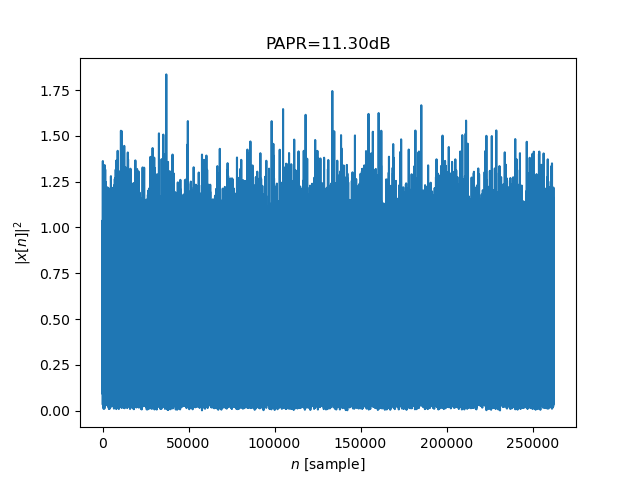
Before running Monte Carlo simulations, we evaluate the PAPR of a single OFDM signal and plot its instantaneous power. The computed PAPR value is displayed in the figure title.
# evaluate PAPR for one signal
N = N_sc*os*L
y = chain(2**16)
y = np.ravel(y, order="F") # perform parallel2serial conversion

papr_dB = compute_PAPR(y, unit="dB", axis=0)
plt.plot(np.abs(y))
plt.ylabel("$|x[n]|^2$")
plt.xlabel("$n$ [sample]")
plt.title(f"PAPR={papr_dB:.2f}dB")
This produces a figure similar to:
Monte Carlo Simulation of CCDF#
We now perform a Monte Carlo simulation to estimate the CCDF of the PAPR for two configurations (256 and 1024 subcarriers). For each case, we compare the simulation results with the theoretical CCDF:
plt.figure()
N_sc_list = [256, 1024]

for N_sc in tqdm(N_sc_list):

    # set S2P and carrier allocation
    carrier_type = np.zeros(os*N_sc)
    carrier_type[:N_sc] = 1

    chain["s2p"].set_N_sub(N_sc)
    chain["carrier_allocator"].set_carrier_type(carrier_type)

    # generate data
    N = N_sc*os*L
    y = chain(N)

    # evaluate metric
    papr_dB_array = compute_PAPR(y, unit="dB", axis=0)

    # display experimental curves
    papr_dB, ccdf = compute_ccdf(papr_dB_array)
    plt.semilogy(papr_dB, ccdf, label=f"exp: N_sc={N_sc}")

    # display theoretical curves
    ccdf_theo = 1 - (1 - np.exp(-gamma))**(N_sc*os)
    plt.semilogy(papr_dB_threshold, ccdf_theo, label=f"theo: N_sc={N_sc}")


plt.ylim([1e-4, 1])
plt.xlim([6, 13])
plt.xlabel("PAPR (dB)")
plt.ylabel("CCDF")
plt.title("CCDFs of PAPR of an OFDM signal with 256 and 1024 subcarriers")
plt.grid()
plt.legend()
The theoretical CCDF is given by:
where \(\gamma\) is the normalized PAPR threshold.
The resulting figure displays both the experimental and theoretical CCDFs for
N_sc = 256 and N_sc = 1024 subcarriers.
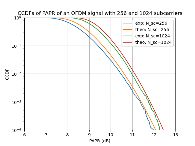
As expected, the probability of large PAPR values increases with the number of subcarriers. For example, with 1024 subcarriers and an oversampling factor of 4, a PAPR around 12 dB is typically observed at CCDF = 10⁻³.
Conclusion#
You have successfully simulated the PAPR of an OFDM signal and compared experimental results with theoretical CCDFs.
You have learned how to:
Define an OFDM chain with adjustable parameters.
Compute the PAPR of a single OFDM waveform.
Estimate the CCDF of the PAPR through Monte Carlo simulation.
Compare simulation results with theoretical benchmarks.
Key takeaway: OFDM signals exhibit high PAPR (around 10-13 dB depending on system size), which motivates PAPR reduction techniques such as clipping, coding, or tone reservation.