Monte Carlo Simulation over AWGN Channel

In this tutorial, we simulate a communication chain with comnumpy and evaluate its Symbol Error Rate (SER) over a range of Signal-to-Noise Ratios (SNRs). Using a Monte Carlo simulation, the chain is executed repeatedly at each SNR value and the experimental results are compared with theoretical predictions.

What you’ll learn:

• How to run a Monte Carlo simulation over a range of SNR values.

• How to compute experimental and theoretical SER for QAM over AWGN.

• How to plot standard SER performance curves on a logarithmic scale.

Introduction

Prerequisites

Make sure you have the following Python libraries installed:

numpy
matplotlib
comnumpy
tqdm

Import Libraries

We start by importing the necessary libraries:

import numpy as np
import matplotlib.pyplot as plt
from tqdm import tqdm
from comnumpy.core import Sequential, Recorder
from comnumpy.core.generators import SymbolGenerator
from comnumpy.core.mappers import SymbolMapper, SymbolDemapper
from comnumpy.core.utils import get_alphabet
from comnumpy.core.channels import AWGN
from comnumpy.core.metrics import compute_ser, compute_metric_awgn_theo

Define Parameters

Next, we set the simulation parameters: modulation order, number of transmitted symbols, and the SNR range to sweep.

M = 16
N = 1000000
modulation = "QAM"
alphabet = get_alphabet(modulation, M)
snr_dB_list = np.arange(0, 22)

AWGN Communication Chain

Define Chain

We define the communication chain using the Sequential object. The chain includes symbol generation, mapping, transmission over an AWGN channel, and symbol demapping.

# create chain
chain = Sequential([
    SymbolGenerator(M),
    Recorder(name="recorder_tx"),
    SymbolMapper(alphabet),
    AWGN(unit="snr_dB", name="awgn_channel"),
    SymbolDemapper(alphabet),
    ])

The processors are:

• SymbolGenerator Generates a stream of integer-valued symbols to transmit.

• Recorder Captures the transmitted symbols for later analysis.

• SymbolMapper Maps integers to QAM constellation points.

• AWGN Simulates the effect of noise for a given SNR value (here expressed in dB).

• SymbolDemapper Maps received noisy constellation points back to integers.

Monte Carlo Simulation

We perform a Monte Carlo simulation over the entire SNR range. At each SNR value, we update the AWGN processor, run the chain, and compute the experimental SER.

# perform monte Carlo simulation
ser_array = np.zeros(len(snr_dB_list))

for index, snr_dB in enumerate(tqdm(snr_dB_list)):

    # change simulation parameters
    chain["awgn_channel"].value = snr_dB

    # run chain
    y = chain(N)

    # evaluate metrics
    data_tx = chain["recorder_tx"].get_data()
    ser = compute_ser(data_tx, y)

    # save and display metrics
    ser_array[index] = ser

Theoretical SER

For comparison, we also compute the theoretical SER curve for QAM modulation over AWGN.

# compute theoretical SER metric
snr_per_bit = (10**(snr_dB_list/10))/np.log2(M)
ser_theo_array = compute_metric_awgn_theo(modulation, M, snr_per_bit, "ser")

Results and Visualization

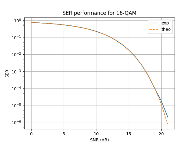
Finally, we plot the experimental and theoretical SER curves. A logarithmic (semilogy) scale is used for the SER axis, which is the standard representation for error rate curves in digital communications.

plt.semilogy(snr_dB_list, ser_array, label="exp")
plt.semilogy(snr_dB_list, ser_theo_array, "--", label="theo")
plt.xlabel("SNR (dB)")
plt.ylabel("SER")
plt.title(f"SER performance for {M}-{modulation}")
plt.legend()
plt.grid()
plt.show()

Conclusion

You have completed a Monte Carlo simulation of SER performance for a QAM-modulated communication system over an AWGN channel.

You have learned how to:

• Build a chain with modulation, channel, and demodulation.

• Run Monte Carlo experiments over a range of SNR values.

• Compare experimental results with theoretical benchmarks.

• Plot standard SER performance curves.

From here, you can:

• Experiment with different modulation orders (e.g., 4-QAM, 64-QAM).

• Extend the chain with channel coding or more realistic channel models.

• Increase the number of transmitted symbols to improve SER estimation accuracy.