MIMO Chain Tutorial#
This tutorial demonstrates how to simulate a MIMO (Multiple-Input Multiple-Output) communication system using the comnumpy library. You will learn how to:
Build a MIMO simulation chain with Rayleigh fading.
Visualize received and equalized signals.
Compare detection algorithms (ZF, MMSE, OSIC, ML).
Perform a Monte Carlo evaluation of Symbol Error Rate (SER).
This tutorial is suited for engineers and students learning about MIMO systems, combining practical examples with theoretical background.
Introduction#
Prerequisites#
Ensure you have the following Python libraries installed:
numpy
matplotlib
comnumpy
Simulation Setup#
Import Libraries#
We start by importing the required libraries and comnumpy components:
import numpy as np
import numpy.linalg as linalg
import matplotlib.pyplot as plt

from tqdm import tqdm
from comnumpy.core import Sequential, Recorder
from comnumpy.core.generators import SymbolGenerator
from comnumpy.core.mappers import SymbolMapper
from comnumpy.core.metrics import compute_ser, compute_ber
from comnumpy.core.utils import get_alphabet
from comnumpy.mimo.channels import FlatMIMOChannel, AWGN
from comnumpy.mimo.utils import rayleigh_channel
from comnumpy.mimo.detectors import MaximumLikelihoodDetector, LinearDetector, OrderedSuccessiveInterferenceCancellationDetector
Define System Parameters#
We define the number of transmit/receive antennas, the modulation order (PSK), and the noise variance:
# Parameters
N = 1000
N_r, N_t = 3, 2
M = 4
alphabet = get_alphabet("PSK", M)
M = len(alphabet)
sigma2 = 0.1
H = rayleigh_channel(N_r, N_t)
The modulation alphabet is automatically generated from the given parameters.
Build the MIMO Chain#
We create a transmission chain consisting of a symbol generator, symbol mapper, and Rayleigh fading channel:
# construct chain
chain = Sequential([SymbolGenerator(M),
                    Recorder(name="data_tx"),
                    SymbolMapper(alphabet),
                    FlatMIMOChannel(H, name="channel"),
                    AWGN(sigma2, name="noise")
                    ])
Y = chain((N_t, N))
This simulates a MIMO transmission over a flat-fading channel with additive Gaussian noise. The received signal is described by:
One-Shot Simulation#
Visualize the Received Signal#
Let’s inspect the received signal on each receive antenna:
# extract signals
S_tx = chain["data_tx"].get_data()

# Figure 1: received signal
fig1, axes1 = plt.subplots(nrows=1, ncols=N_r, figsize=(4 * N_r, 4))
for num_channel in range(N_r):
    y = Y[num_channel, :]
    ax = axes1[num_channel]
    ax.plot(np.real(y), np.imag(y), ".")
    ax.set_title(f"Received signal (antenna {num_channel+1})")
    ax.set_aspect("equal", adjustable="box")
    ax.set_xlim([-2, 2])
    ax.set_ylim([-2, 2])
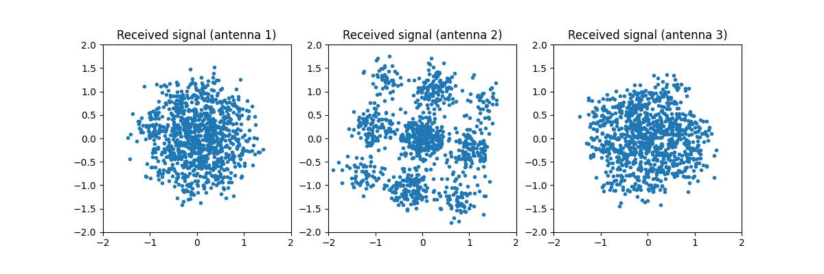
You should observe that the received signal consists of noisy superpositions of multiple transmitted streams.
Zero-Forcing Equalization#
We now apply Zero-Forcing (ZF) equalization using the pseudo-inverse of the channel matrix:
# ZF equalization
H_inv = linalg.pinv(H)
X_est = np.matmul(H_inv, Y)
This separates the transmitted streams assuming perfect channel knowledge while ignoring noise enhancement. The ZF-equalized symbols are given by
Visualize the Estimated Symbols#
We plot the ZF-equalized symbols:
# Figure 2: estimated signal
fig2, axes2 = plt.subplots(nrows=1, ncols=N_t, figsize=(4 * N_t, 4))
for num_channel in range(N_t):
    x_est = X_est[num_channel, :]
    ax = axes2[num_channel]
    ax.plot(np.real(x_est), np.imag(x_est), ".")
    ax.set_title(f"Estimated signal (antenna {num_channel+1})")
    ax.set_aspect("equal", adjustable="box")
    ax.set_xlim([-2, 2])
    ax.set_ylim([-2, 2])
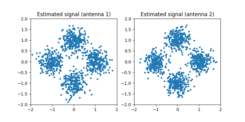
The estimated points should cluster around the ideal constellation points, although residual noise remains visible.
Detection Comparison#
We now compare four MIMO detection strategies:
ML: Maximum Likelihood
ZF: Zero-Forcing
MMSE: Minimum Mean Square Error
OSIC: Ordered Successive Interference Cancellation
All four detectors are available in comnumpy.
# evaluate the BER for several detectors
detector_list = [
    LinearDetector(alphabet, H, method="zf", name="ZF"),
    LinearDetector(alphabet, H, sigma2=sigma2, method="mmse", name="MMSE"),
    OrderedSuccessiveInterferenceCancellationDetector(alphabet, "sinr", H, sigma2=sigma2, name="OSIC"),
    MaximumLikelihoodDetector(alphabet, H, name="ML")
    ]
for detector in detector_list:
    S_est = detector(Y)
    ser = compute_ser(S_tx, S_est)
    name = detector.name
    print(f"* detector {name}: ser={ser}")
Each detector is tested on the same channel realization, and the SER is printed. Typical output:
detector ZF: ser=0.005
detector MMSE: ser=0.004
detector OSIC: ser=0.001
detector ML: ser=0.0005
Monte Carlo Evaluation#
To get a more reliable estimate of the SER, we run a Monte Carlo simulation.
# perform monte carlo simulation
snr_dB_list = np.arange(0, 20, 2)
N_test = 1000
ser_data = np.zeros((len(snr_dB_list), len(detector_list)))

for index_snr, snr_dB in enumerate(tqdm(snr_dB_list)):
    sigma2 = N_t * (10**(-snr_dB/10))
    chain["noise"].value = sigma2

    # update sigma2 for the MMSE and OSIC detector
    detector_list[1].sigma2 = sigma2
    detector_list[2].sigma2 = sigma2

    for trial in range(N_test):

        # new channel realization
        H = rayleigh_channel(N_r, N_t)
        chain["channel"].H = H

        # generate data
        Y = chain((N_t, N))
        S_tx = chain["data_tx"].get_data()

        # test detector
        for index, detector in enumerate(detector_list):

            # update channel information
            detector.H = H
            # perform detection
            S_est = detector(Y)
            # evaluate metrics
            ser_data[index_snr, index] += compute_ser(S_tx, S_est)

    ser_data[index_snr, :] /= N_test
This simulates multiple random channels and noise realizations for a range of SNR values.
Plot SER vs SNR#
Finally, we plot the SER for each detection scheme as a function of SNR:
# plot figures
plt.figure()
for index, detector in enumerate(detector_list):
    plt.semilogy(snr_dB_list, ser_data[:, index], label=detector.name)
plt.ylabel("SER")

plt.xlabel("SNR (dB)")
plt.xlim([0, 20])
plt.ylim([10**-3, 1])
plt.legend()
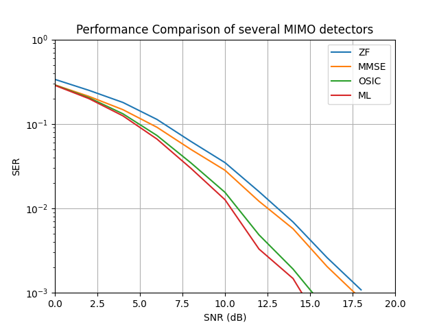
This figure compares detection methods as a function of SNR. The maximum-likelihood (ML) detector delivers the best performance, albeit at higher computational cost, while the OSIC detector performs close to ML.
Conclusion#
This tutorial highlighted:
How to simulate a MIMO transmission with
comnumpy.How ZF equalization recovers the signal from a multi-stream mixture.
How various MIMO detectors compare under different SNR conditions.
Why advanced detection schemes like OSIC and ML outperform linear methods in challenging channel conditions.
With comnumpy, you can rapidly prototype, test, and visualize MIMO systems for research, teaching, or self-study.