
Monte Carlo Simulation over AWGN Channel#
One run of a chain gives one error rate at one SNR. A performance figure needs a curve, so the chain has to be run again at every operating point – that repetition is what “Monte Carlo simulation” means, and there is nothing more to it than a loop.
We will write that loop by hand first, because it is worth seeing exactly
what a sweep is made of. Then we will replace it with
monte_carlo(), which does the same four things in
one call, and use that in every tutorial that follows.
Note
Before you start. This tutorial follows First Simulation, which built a chain and ran it once. Here we run it many times, which is what a performance figure is made of.
What you’ll learn:
How to reconfigure a chain between runs with
set_params, and make each run reproducible withseed.How to write a Monte Carlo loop, and then how to replace it with
monte_carlo.How to write the closed form a measured curve should follow, evaluate it in plain NumPy, and then get the same numbers from the constellation itself.
How to draw the result with
plot_error_rate, the figure this library uses for every error rate.How to compare modulation orders fairly, at equal energy per bit.
Introduction#
Prerequisites#
Make sure you have the following Python libraries installed:
numpy
scipy
matplotlib
comnumpy
Import Libraries#
We start by importing the necessary libraries:
import numpy as np
import matplotlib.pyplot as plt
from functools import partial
from scipy.special import erfc
from comnumpy import monte_carlo, print_data
from comnumpy.core import Sequential
from comnumpy.core.generators import SymbolGenerator
from comnumpy.core.mappers import SymbolMapper, SymbolDemapper
from comnumpy.core.utils import Constellation, ebn0_to_snr_dB
from comnumpy.core.channels import AWGN
from comnumpy.core.metrics import compute_ser, compute_ber
from comnumpy.core.visualizers import plot_error_rate
from comnumpy import style

style.use()

img_dir = "../../docs/tutorials/img/"
Define Parameters#
Next, we set the simulation parameters: the number of transmitted symbols, the constellation, and the SNR range to sweep. The constellation is one object – it carries the alphabet the mapper needs, its order, and the closed form we compare against below.
# parameters
N = 1000000
constellation = Constellation("QAM", 16)
snr_dB_list = np.arange(0, 22)
AWGN Communication Chain#
Define Chain#
We define the communication chain using the Sequential object.
The chain includes symbol generation, mapping, transmission over an AWGN channel,
and symbol demapping. It is written as a function because the last section of
this page builds one per constellation order.
# One chain, transmitter to decision. Every block that a sweep must
# reconfigure is named: the channel for the SNR, the generator, mapper
# and demapper for the constellation the last section changes.
chain = Sequential([
    SymbolGenerator(constellation.order, name="tx"),
    SymbolMapper(constellation, name="mapper"),
    AWGN(snr_dB=0, name="awgn_channel"),
    SymbolDemapper(constellation, name="demapper"),
], observations=["tx"])
The processors are:
SymbolGeneratorGenerates a stream of integer-valued symbols to transmit. It is named"tx"so the sweep can compare the chain output against the transmitted symbols (seereference="tx"below).SymbolMapperMaps integers to QAM constellation points.AWGNSimulates the effect of noise for a given SNR value (here expressed in dB).SymbolDemapperMaps received noisy constellation points back to integers.
Monte Carlo Simulation#
Start with the loop you would write yourself. At each SNR value there are exactly four things to do: reseed the chain so the run is reproducible, reconfigure the block that has to change, run it, and measure against the transmitted symbols.
# A Monte Carlo simulation is three parts, always in this order: the
# metric pre-allocated, the loop that fills it, the display at the end.
# Written out, at three SNR values:
probed_snr_dB = snr_dB_list[::8]
ser_by_hand = np.zeros(len(probed_snr_dB))
for index, snr_dB in enumerate(probed_snr_dB):
    chain.seed(1)
    chain.set_params(awgn_channel__snr_dB=snr_dB)
    detected = chain(N)                  # run first: the observation is filled by it
    ser_by_hand[index] = compute_ser(chain.observation("tx"), detected)
Three chain services appear there, and they are the ones every study is made of.
seed gives each stochastic block its own child seed, so the same seed
always gives the same signal – a curve you cannot reproduce is a curve you
cannot debug. set_params addresses a block by the name it was given at
construction, with the dotted notation "awgn_channel.snr_dB"; this is why
blocks are named. And the observation returns what the transmitter produced, so the
metric has something to compare against – after the run, never before.
Now the same thing in one call. monte_carlo() takes
the chain, the dotted name of what varies, the values it takes, and the metrics
to collect – and does the reseed, the reconfigure, the run and the measurement
at every point:
# monte_carlo (decision D35) is that loop, and nothing more: the same
# reconfigure-reseed-run-collect, over every point, in one call.
results = monte_carlo(chain, "awgn_channel.snr_dB", snr_dB_list,
                      {"ser": compute_ser}, N, reference="tx", seed=1)
ser_array = results["ser"]

# An abscissa and one series per curve is what a sweep produces, and
# print_data is what shows it: the same dictionary would draw the figure.
print_data({"x": probed_snr_dB,
            "curves": {"loop": ser_by_hand,
                       "monte_carlo": ser_array[::8]}},
           xlabel="SNR [dB]", ylabel="SER")
SER
SNR [dB]     loop  monte_carlo
------------------------------
       0  0.74057      0.74105
       8  0.35345      0.35331
      16  0.00724      0.00712
The two are the same computation. They do not print the same digits because
monte_carlo gives each point its own child seed rather than reseeding every
point to the same value, so the noise realizations differ; the gap is the
Monte Carlo error of a million symbols, not a difference of method.
From here on, the other tutorials use monte_carlo without rewriting the
loop. When you see it sweeping a channel matrix rather than an SNR (in
MIMO Chain Tutorial and Alamouti Space-Time Coding Tutorial), it is still these four steps – only the
parameter that varies has changed.
Theoretical SER#
A measured curve is worth little on its own. What makes it a result is the curve it is supposed to lie on.
The closed form#
A square \(M\)-QAM constellation is the Cartesian product of two independent \(\sqrt{M}\)-PAM constellations, one on each quadrature. With \(k = \log_2 M\) bits per symbol, the signal-to-noise ratio per bit \(\gamma_b = E_b/N_0\) and the Gaussian tail function
the error probability of one PAM component is
A symbol is received correctly only when both components are, so the symbol error probability is
This is the standard result; see Proakis and Salehi [Proakis2008], Section 4.3.
Note which SNR parameterizes it: the expression is written against
\(\gamma_b\), the ratio per bit, whereas AWGN(snr_dB=) takes a symbol
SNR \(\gamma_s = k\gamma_b\). Getting that wrong moves the curve by
\(10\log_{10} k\) dB – 6 dB for 16-QAM – with nothing to signal it.
In NumPy, written out#
There is no machinery in this. scipy.special.erfc gives \(Q\), and the
two expressions above transcribe line for line:
def qfunc(x):
    """Gaussian tail function, the one the textbooks write as Q."""
    return 0.5 * erfc(x / np.sqrt(2))


# The closed form of Proakis, written out. A square M-QAM is two
# independent sqrt(M)-PAM constellations, so a symbol is correct only
# when both components are. AWGN(snr_dB=) is a symbol SNR and the
# expression is parameterized by the SNR per bit, hence the division by k.
M = constellation.order
k = int(np.log2(M))
gamma_b = 10 ** (snr_dB_list / 10) / k
P_pam = 2 * (1 - 1 / np.sqrt(M)) * qfunc(np.sqrt(3 * k * gamma_b / (M - 1)))
ser_theo_array = 1 - (1 - P_pam) ** 2
From the constellation#
The same expression is already in the library, and the constellation knows
which one applies to it: it carries its family and its order, so the theory
cannot end up describing a modulation other than the one the chain transmits.
per="symbol" says that the swept SNR is the symbol SNR, and the division
by \(k\) above happens inside.
# The same expression is already in the library, and the constellation
# knows which one applies to it. per="symbol" says that the swept SNR is
# the symbol SNR, and the conversion to Eb/N0 above happens inside.
from_object = constellation.metrics(snr_dB_list, per="symbol")["ser"]
gap = np.max(np.abs(ser_theo_array - from_object))
print(f"largest gap between the two closed forms: {gap:.3e}")
largest gap between the two closed forms: 3.331e-16
Machine precision – they are the same formula. From here on we call the method, which is one line instead of five and cannot describe the wrong modulation.
Results and Visualization#
An error rate curve is always drawn the same way, so the library draws it for
you: plot_error_rate puts the measurements as hollow markers and the
closed form as a line of the same colour, on a logarithmic ordinate with a
grid on both decades. A measurement and the theory it is being compared with
share a colour, so a pair reads as one statement.
# as a line of the same colour: the figure every sweep ends with
label = f"{constellation.order}-{constellation.family}"
plot_error_rate(snr_dB_list, {label: ser_array},
                theory={label: ser_theo_array},
                ylabel="SER", title=f"SER performance for {label}")
plt.savefig(f"{img_dir}/monte_carlo_awgn.png")
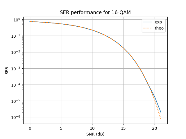
The markers sit on the line over five decades. The last point, at 21 dB, is an SER of \(10^{-6}\) measured from \(10^6\) symbols – one error. It is on the curve by luck as much as by physics, and it is the point at which this sweep has run out of samples rather than out of accuracy.
Comparing modulation orders#
One constellation against its own theory says the simulation is right. It does not say what a constellation is worth. For that, several orders have to be put on the same axes – and the choice of that axis is the whole question.
At equal \(E_s/N_0\), a dense constellation is unduly favoured: it spends
the same energy per symbol while carrying more bits. The fair comparison is at
equal energy per bit, \(E_b/N_0\), which is why
ebn0_to_snr_dB() exists. The conversion needs
\(k\) – chain-level knowledge the channel block does not have and should
not guess (decision D41), so it happens at the call site:
# energy per symbol a dense constellation is favoured, because it spends
# the same energy on more bits. ebn0_to_snr_dB does that conversion, and
# it needs k, which is chain-level knowledge the channel does not have.
ebn0_dB_list = np.arange(0, 25, 2)
N_compare = 100000
orders = np.array([4, 16, 64, 256])
bits_per_symbol = np.log2(orders).astype(int)     # vectorized, not a loop
curves = {}
theory = {}
for index, order in enumerate(orders):
    other = Constellation("QAM", int(order))
    bits = int(bits_per_symbol[index])
    snr_dB_values = ebn0_to_snr_dB(ebn0_dB_list, bits_per_symbol=bits)
    # the same chain, reconfigured (D50): set_params re-runs the
    # coercions a bare assignment would skip
    chain.set_params(tx__M=other.order, mapper__alphabet=other,
                     demapper__alphabet=other)
    collected = monte_carlo(chain, "awgn_channel.snr_dB",
                            snr_dB_values,
                            {"ber": partial(compute_ber, width=bits)},
                            N_compare, reference="tx", seed=1)
    order_label = f"{order}-QAM"
    curves[order_label] = collected["ber"]
    theory[order_label] = other.metrics(ebn0_dB_list, per="bit")["ber"]
The metric changes with the axis. Against \(E_b/N_0\) the natural quantity
is the bit error rate, and compute_ber needs the symbol width, which
functools.partial supplies once per order.
The reference curve is no longer exact here, and the figure shows it. The BER of the closed form is the Gray-mapping approximation \(P_b \simeq P_s / k\), which assumes a symbol error corrupts exactly one bit out of \(k\) – true when the wrong decision is a nearest neighbour, false when the noise is large enough to reach further. So the markers sit above the line at the left of the figure, by 17 % for 16-QAM and by a factor 2.2 for 256-QAM at 0 dB, and settle onto it as the error rate falls: below \(10^{-2}\) the two agree to within a few percent for every order. This is an approximation behaving as documented, not a simulation disagreeing with theory.
ax = plot_error_rate(ebn0_dB_list, curves, theory=theory,
                     xlabel="$E_b/N_0$ [dB]", ylabel="BER",
                     title="Square QAM at equal energy per bit")
# The closed forms run down to 1e-12; the measurements cannot follow them
# past a few 1e-6, so the axis stops where the simulation stops speaking.
ax.set_ylim(1e-6, 1)
plt.savefig(f"{img_dir}/monte_carlo_awgn_orders.png")
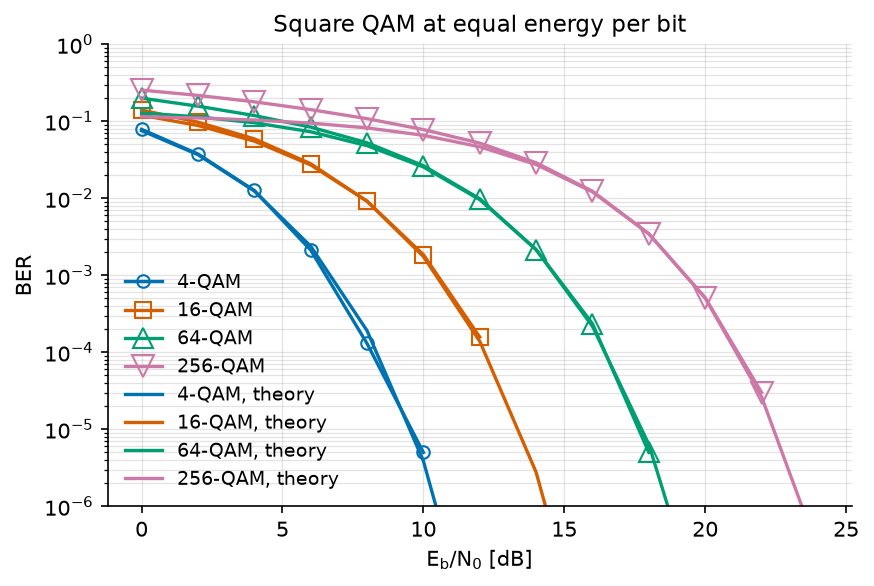
The waterfalls are almost evenly spaced: each doubling of the bits per symbol shifts the curve by 4 to 5 dB of energy per bit, read directly off the figure. That price is what the rest of a communication system is built to negotiate: coding buys some of it back (Channel Coding), shaping buys a little more (Probabilistic Shaping), and a channel that is not simply AWGN changes the terms entirely (OFDM Tutorial).
The measured curves stop where the estimator does. Each point here is 100 000
symbols, so a 4-QAM run has 200 000 bits and cannot resolve a BER below about
\(5 \times 10^{-6}\); plot_error_rate drops the points where no error
was seen rather than drawing them at zero, and the axis stops at
\(10^{-6}\) for the same reason. Reading a curve past its own floor is the
most common way to publish a wrong figure.
Conclusion#
You have turned one run into a curve, checked it against a closed form you wrote yourself, and used it to price four modulation orders against each other.
You have learned how to:
Reconfigure and reseed a chain between runs.
Collect a metric over a range of parameter values, by hand and with
monte_carlo.Write a theoretical error rate in NumPy, and get the same numbers from the constellation.
Read a measured curve against a closed form, and know where it stops being readable.
Compare modulations at equal energy per bit.
From here, OFDM Tutorial keeps the chain and changes the channel: instead of one noise term, the signal arrives several times, and the receiver has to undo that. Two ways of doing so, at very different prices.
References#
J. G. Proakis and M. Salehi, Digital Communications, 5th ed., McGraw-Hill, 2008. Section 4.3, symbol and bit error probabilities for PAM, PSK and QAM over the AWGN channel.