Profiling a Communication Chain

In this tutorial, you will learn how to profile a communication chain using comnumpy. Profiling measures the computational cost of each processor, helping you identify performance bottlenecks in complex simulations.

You will build an OFDM communication chain with channel effects, run the simulation, and visualize the profiling results.

What you’ll learn:

• How to build an OFDM communication chain with channel effects.

• How to use plot_chain_profiling to measure per-processor execution time.

• How to identify computational bottlenecks in a simulation chain.

Introduction

Import Libraries

We start by importing the necessary libraries:

import numpy as np
import matplotlib.pyplot as plt
from comnumpy.core import Sequential, Recorder
from comnumpy.core.generators import SymbolGenerator
from comnumpy.core.mappers import SymbolMapper, SymbolDemapper
from comnumpy.core.channels import AWGN, FIRChannel
from comnumpy.core.processors import Serial2Parallel, Parallel2Serial
from comnumpy.core.utils import get_alphabet
from comnumpy.core.metrics import compute_ser
from comnumpy.core.visualizers import plot_chain_profiling
from comnumpy.ofdm.processors import CarrierAllocator, FFTProcessor, IFFTProcessor, CyclicPrefixer, CyclicPrefixRemover, CarrierExtractor
from comnumpy.ofdm.compensators import FrequencyDomainEqualizer
from comnumpy.ofdm.utils import get_standard_carrier_allocation

Define Parameters

Next, we define the communication and channel parameters:

# parameters
modulation = "QAM"
M = 16          # Modulation order
N_h = 5         # Number of channel taps
N_cp = 10       # Cyclic prefix length
N = 100000      # Number of symbols
sigma2 = 0.01   # Noise variance

alphabet = get_alphabet(modulation, M)  # Get alphabet for QAM modulation
carrier_type = get_standard_carrier_allocation("802.11ah_128")  # Standard carrier allocation

# extract carrier information
N_carriers = len(carrier_type)
N_carrier_data = np.sum(carrier_type == 1)  # Number of data carriers
N_carrier_pilots = np.sum(carrier_type == 2)  # Number of pilot carriers

# channel parameters
h = 0.1 * (np.random.randn(N_h) + 1j * np.random.randn(N_h))
h[0] = 1
pilots = 10 * np.ones(N_carrier_pilots)  # Pilot values

OFDM Communication Chain

Define the Chain

We build a complete OFDM chain using the Sequential object. This chain includes mapping, carrier allocation, IFFT/FFT processing, cyclic prefix handling, channel effects, equalization, and demapping.

chain = Sequential([
    SymbolGenerator(M),
    SymbolMapper(alphabet),
    Serial2Parallel(N_carrier_data),
    CarrierAllocator(carrier_type=carrier_type, pilots=pilots),
    IFFTProcessor(),
    CyclicPrefixer(N_cp),
    Parallel2Serial(),
    FIRChannel(h),
    AWGN(sigma2),
    Serial2Parallel(N_carriers + N_cp),
    CyclicPrefixRemover(N_cp),
    FFTProcessor(),
    FrequencyDomainEqualizer(h=h),
    CarrierExtractor(carrier_type),
    Parallel2Serial(),
    SymbolDemapper(alphabet)
])

The chain is composed of the following processors:

• SymbolGenerator Generates a sequence of integer-valued symbols to transmit.

• SymbolMapper Maps integers to QAM constellation points.

• Serial2Parallel / Parallel2Serial Reshape data between serial and parallel streams, as required by OFDM processing.

• CarrierAllocator Assigns data and pilot symbols to their designated subcarriers.

• IFFTProcessor / FFTProcessor Perform the Inverse Fast Fourier Transform and Fast Fourier Transform operations, respectively.

• CyclicPrefixer / CyclicPrefixRemover Add and remove the cyclic prefix to prevent inter-symbol interference.

• FIRChannel Models a frequency-selective multipath channel.

• AWGN Adds white Gaussian noise.

• FrequencyDomainEqualizer Compensates for channel distortion in the frequency domain.

• CarrierExtractor Extracts data and pilot carriers after equalization.

• SymbolDemapper Maps received constellation points back to integer symbols.

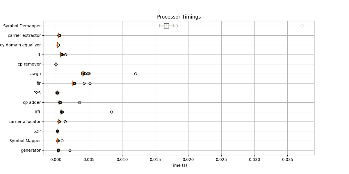
Profiling the Chain

To profile the chain, we use the plot_chain_profiling function. This function measures the execution time of each processor for a given input size and produces a bar chart of the results.

# profiling chain
plot_chain_profiling(chain, input=N)

The resulting figure shows the time spent in each processor, making it easy to identify which stages dominate the computation.

Conclusion

You have successfully profiled an OFDM communication chain with comnumpy.

Profiling is a powerful tool to:

• Detect computational bottlenecks in complex simulations.

• Compare the efficiency of different processors or chain configurations.

• Optimize large-scale communication scenarios.

From here, you may want to explore:

• Profiling different modulation schemes or OFDM sizes.

• Comparing different equalization techniques.

• Combining profiling with performance metrics such as SER or BER.